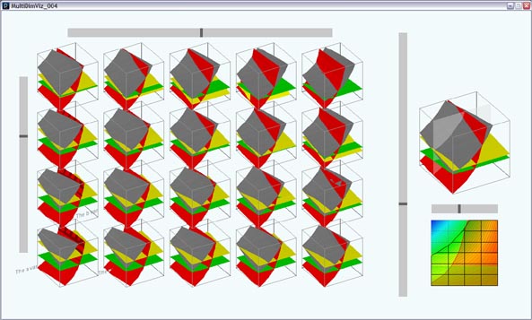
For a while I've been interested in visualisation of data.  It's something that I have to deal with every day at work and I've tried to learn from many of the people active in this field, not least Ben Fry (one of the creators of Processing and author of the excellent "Visualizing Data") and Edward R Tufte (if you're interested in this data visualisation I would recommend you buy all his beautiful books)

My main problem is this: how can I see the response of a system (in my case an aircraft concept design) when I change its inputs? It's not an uncommon problem by any means but for me the complexity comes from the number of inputs and outputs that I'd like to be able to see & understand.

In my work I can generally expect to use at least two inputs but more often three inputs.  While I will only need to see one main output,  there will also be many other supplementary outputs (in the form of constraints: valid and invalid areas) on the same range of inputs.

I'm pretty sure that this problem has been solved elsewhere and I'd love to be told about other people's solutions, but I was also curious about what I might learn if I tried to solve the problem. In the end it was an interesting journey...

Programming

I turned to Processing and set up a few approaches (I'll release the code when I can get it beaten into shape) and I managed to get two visualisation approaches for 3D/4D datasets (three to four independent input variables, 1 output).  Neither of these were new (arrays of carpet plots and contour plots), I'll describe them if people are interested.

However, I wanted to see how many dimensions I could get an interactive visualisation to work for, in the end I managed one that would allow five.

I used multiple copies of a volume plot (a 3D contour plot), also called an isosurface, to display the data.  

An isosurface is a 3D analogue of the isolines seen on a contour plot, it is a surface representing all the points in 3D space where a value is constant.  They are often used in aircraft design (amongst other places) to visualise the results of CFD (Computational Fluid Dynamics) calculations where they one might used to represent the boundary between sub- and super- sonic flow, for example.

With an isosurface I can display the three input variables on the three spatial dimensions of the plot (up/down, left/right, in/out), I can then display the result using an isosurface.  In some ways this won't be ideal because, unlike a contour plot, I can now only see one value of output at a time (like seeing only 1 contour line, although in the end this turns out not to be a problem for me at least) unless I go to partially transparent approaches which were slow and didn't work that well for me.

Constraints - the parts you can't use

The display of constraints on charts is important for the use of data in aircraft concept design and sizing.  

Generally data produced during an aircraft sizing trade (a scan through a set of inputs) will produce points that do not meet all of the aircraft's requirements (takeoff performance, time taken to climb to altitude, approach speed etc.)

This means that it is necessary to find ways to show which points do not meet (or which over meet) the requirements. Interpolation allows the behaviour of the constraints to be estimated in unsampled regions between data points.

I can also use isosurfaces to display my constraints, I just need to overlay the main response with the secondary constraint response isosurfaces (where the constraint is just met) and I was easily able to display the valid/invalid regions.

I ended up with something that looks like this:

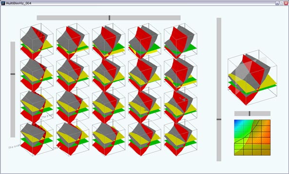
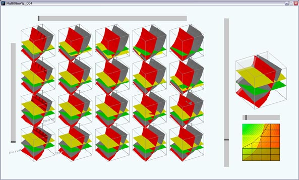
The first three independent variables are displayed on the three axes of each isosurface plot.  The main response is the grey surface, the value of the output that is used to generate the grey surface is controlled by the vertical slider on the right.  It's possible to change the displayed value by moving the slider interactively and so can, by inspection, find the best points in any plot.  The best point in this case is constrained by the red, green and yellow constraint surfaces.  For the sake of argument we may assume that the valid space is above them (although the plots may be rolled and rotated together for a clear view).

The sliders on the top and left side represent where in the range of the fourth and fifth variables we are most interested and control interpolation of the data at these values.  This interpolated data is displayed on the larger repeater plot on the right hand side.  In the example below we are looking at the data around the middle of the range of the fourth variable (across) and about a quarter of the way down the fifth (down):

The repeater is further downsampled using the smallest horizontal slider which gives a cross section of the repeater isosurface on a conventional contour plot.  Here I've tried to find the best (in this case lowest) unconstrained point in the range, it's at the lower right:

Conclusions

Is it easy to use? Well, sort of. I don't find it a problem and in a couple of cases it has been really useful - I suppose I've got used to it.  I don't think that I'll ever use it to explain a dataset to anyone else though and it's a lot clearer used interactively, pictures of it don't really make it easy to see the way that the data changes through the range but as a proof of concept it was really interesting to work on.

I learned:

• How to make volume plots (I wrote my own implementation of the marching tetrahedrons algorithm - in fact I deduced it independently from scratch before I knew it existed, thought I was a genius then realised it had existed for 30 years already and felt silly)
• How to make contour plots using marching squares